Monthly, quarterly and annual growth rates
I received the following question by email:
I was wondering if mathematical relationships exist between monthly, quarterly, and annual growth rates (percentage changes). For time series data …
1) Is there a mathematical formula to know by how many months the Month-to-Month changes lead turns in this-month-to-the-same-month-one-year-ago changes (annual changes)?
2) Is there a mathematical formula to know by how many quarters the Quarter-to-Quarter changes lead turns in this-quarter-to-the-same-quarter-one-year-ago changes (annual changes)?
Also, regarding simple moving averages/totals:
3) Is there an exact or approximate formula to know by how many months a 3-month simple moving average (or moving total) leads a turn in a 12-month simple moving average (or moving total)?
As an example: Inflation is typically measured with Y/Y percentage changes in the CPI. So, it would be helpful to be able to identify when the 12-month rate of change will likely reach a top or bottom, using the 1-month or 3-months rates of change.
Monthly growth vs year-over-year growth
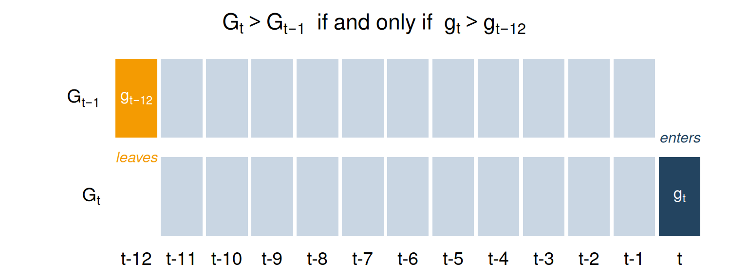
Suppose we have monthly data y_1,y_2,\dots. Then the monthly growth rates are given by g_t = \frac{y_t - y_{t-1}}{y_{t-1}}, and the year-over-year growth rates are given by G_t = \frac{y_t - y_{t-12}}{y_{t-12}}. A little algebra gives 1 + G_t = \prod_{j=1}^{12} (1 + g_{t-j+1}). \tag{1} So the year-over-year rate is the compounded product of the last 12 monthly rates. This gives a recurrence relationship: \frac{1 + G_t}{1 + G_{t-1}} = \frac{1 + g_t}{1 + g_{t-12}}. Therefore G_t > G_{t-1} \iff g_t > g_{t-12}. In other words, the year-over-year rate rises when the current monthly change exceeds the change 12 months ago, and falls when the reverse holds. Figure 1 shows why: moving from G_{t-1} to G_t, the 12-month window drops g_{t-12} and adds g_t, while the other 11 months are common to both.
For example, annual inflation peaks when the monthly rates entering the 12-month window fall below the rates dropping out of it. Because year-over-year growth is effectively a 12-month trailing window of monthly growth, month-to-month growth tends to lead year-over-year growth by just under half the window length: the centre lag of an equally-weighted k-period trailing window is (k - 1)/2 periods, or 5.5 months when k = 12.
This centre-lag rule works best when monthly growth is smooth and roughly symmetric around its turning points, and is less reliable for noisy series or for turns that are much sharper on one side than the other.
Quarterly growth vs year-over-year growth
The quarterly version is exactly analogous: just replace 12 by 4. Since four-quarter growth is a trailing 4-quarter window of quarterly growth, quarter-to-quarter growth leads year-over-year growth by about 1.5 quarters, under the same condition as above.
Log growth rates
Taking logarithms turns the multiplicative relationship above into a linear one, which is more convenient for compounding over several periods and for forecasting. For small rates, log growth is very close to percentage growth.
Define monthly log growth \ell_t = \ln(1 + g_t) and year-over-year log growth L_t = \ln(1 + G_t), using g_t and G_t from above. Taking logs of Equation 1 turns the product into a sum: L_t = \sum_{j=0}^{11} \ell_{t-j}. So L_t rises when \ell_t > \ell_{t-12}: the same turning condition as before, now linear rather than multiplicative.
This also gives a forecasting formula: L_{t+h} = L_t + \sum_{s=1}^{h} \left( \ell_{t+s} - \ell_{t+s-12} \right). So given a model for future monthly growth, you can forecast the future year-over-year rate in log terms.
Setting h = 3 and shifting back three months compares the most recent 3-month block to the corresponding block a year earlier: L_t - L_{t-3} = \sum_{j=0}^{2} \ell_{t-j} - \sum_{j=0}^{2} \ell_{t-12-j}. So the year-over-year rate has risen over the past three months if the most recent 3-month growth exceeds the same 3-month block a year earlier.
For CPI inflation, y_t is the price index, \ell_t is (approximately) the monthly inflation rate, and L_t is approximately the year-over-year rate quoted in the news, which is the percentage change G_t.
3-month moving averages vs 12-month moving averages
A trailing simple moving average of \{y_1, y_2, \dots\} is defined as: \hat{T}_{k,t} = \frac{1}{k} \sum_{j=0}^{k-1} y_{t-j}. Then \hat{T}_{k,t} - \hat{T}_{k,t-1} = \frac{1}{k} (y_{t} - y_{t-k}). So \hat{T}_{k,t} rises when the newest observation entering the window, y_{t}, exceeds the oldest observation leaving the window, y_{t-k}, and falls when the reverse holds.
As with the growth-rate case, the practical lead between two moving averages of different lengths can be approximated from the centre of each trailing window. A trailing k-period average is centred about (k - 1)/2 periods in the past, so a 3-month average is centred about 1 month in the past, while a 12-month average is centred about 5.5 months in the past. So a 3-month moving average tends to lead a 12-month moving average by about 5.5 - 1 = 4.5 months, for the same reason that monthly growth leads year-over-year growth above. As before, this holds as long as the series moves slowly relative to the 12-month window.
Update (25 October 2026): base effects
The same reader sent a follow-up question:
Inflation is commonly measured with the 12-month (annual) rate of change (ROC) in the Consumer Price Index (CPI). One potential issue with the ROC is that changes in the base period from the past can distort the indicator. Central banks often refer to the so-called “base effects” when talking about such changes taking place in the CPI. Meaning that the change in the 12-month (annual) rate of change is influenced not only by the most recent developments, but also by developments in the same month of the previous year (base period one year earlier). So, the change between periods 13 and 12 matters as well as the change between the two most recent months. Your Figure 1 illustrates this concept well.
What would be a proper way of calculating the contributions of the earlier change (from t-13 to t-12) and the most recent change (from t-1 to t) to the overall 12-month change? Is there a different calculation one can use that will correct or reduce the influence of the base effects so the underlying trend remains intact? For example, would it make sense to use a simple or exponential moving average of 1-month change?
Decomposing the change in the annual rate
In log terms, the decomposition is exact and additive. From L_t = \sum_{j=0}^{11}\ell_{t-j}, L_t - L_{t-1} = \underbrace{\ell_t}_{\text{current month}} - \underbrace{\ell_{t-12}}_{\text{base month}}. So the contribution of the most recent change is \ell_t, and the contribution of the base month is -\ell_{t-12}. The two receive equal weight, with opposite signs, as Figure 1 shows.
In percentage terms, the recurrence relationship above gives G_t - G_{t-1} = \frac{1 + G_{t-1}}{1 + g_{t-12}}\,(g_t - g_{t-12}), which splits exactly into a current contribution \frac{1 + G_{t-1}}{1 + g_{t-12}}\,g_t and a base contribution -\frac{1 + G_{t-1}}{1 + g_{t-12}}\,g_{t-12}. The scaling factor is close to 1 at typical inflation rates, so G_t - G_{t-1} \approx g_t - g_{t-12} is usually accurate enough.
Central banks often use a narrower definition. The ECB distinguishes a technical base effect (the whole contribution of the base month) from an economic one, which is only the part of the base-month change that was unusual, such as an energy price spike or a tax change, relative to its normal seasonal pattern (ECB Monthly Bulletin, January 2005). With seasonally adjusted monthly log growth \ell_t^{SA}, the economic base effect is roughly -(\ell_{t-12}^{SA} - \bar\ell), where \bar\ell is a typical monthly growth rate.
Reducing base effects
The annual rate is already a simple moving average of monthly changes: L_t/12 is the 12-month trailing average of \ell_t. Base effects arise from the rectangular shape of that window. A one-off shock gets full weight for 12 months and then drops out abruptly, causing a jump in the annual rate a year later. So a 12-month simple moving average of monthly changes reproduces the base effects exactly.
Some alternatives do help.
- An exponential moving average of seasonally adjusted monthly changes. With E_t = \alpha\ell_t^{SA} + (1 - \alpha)E_{t-1}, E_t - E_{t-1} = \alpha(\ell_t^{SA} - E_{t-1}). The “base” is now a geometrically weighted average of all past months, rather than a single month a year earlier. Old shocks fade gradually rather than dropping out all at once. The mean lag is (1 - \alpha)/\alpha months, so \alpha \approx 0.15 gives about the same 5.5-month lag as the annual rate. Multiply by 12 to put it on an annual scale.
- Shorter annualised windows, such as 3-month or 6-month annualised growth of seasonally adjusted data. These still have base effects, but from 3 or 6 months back, so they are more timely and also noisier.
- Removing the shocks at source. Base effects are mostly caused by a few volatile items. Trimmed-mean and weighted-median measures exclude the most extreme price changes, so a one-off shock in a single item has less influence on the annual rate, both when it occurs and when it drops out a year later. The RBA uses its trimmed mean measure as a guide to underlying inflation for this kind of reason.
- The growth rate of an estimated trend, for example from an STL decomposition of log CPI. This is smooth, but the estimates at the end of the series are revised as new data arrive.
The exponential moving average must use seasonally adjusted monthly changes. The 12-month window conveniently cancels seasonality, but an exponential moving average of unadjusted changes will not.
Whichever filter is used, there is a trade-off between smoothness and timeliness. No filter reveals the underlying trend without some lag or some uncertainty at the end of the series.